This section describes the various ways available to shape the timing of either the whole animation or groups of selected frames. The controls and functions to edit the timing are enclosed by the Timing-tab of the "Animation editor" group-box:
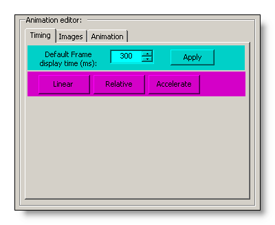
The controls on this tab are organized in two rows (highlighted with different colors in the image above), where each row has it's own logic, on how the timing of individual or groups of frames is affected.
The first row (blue) serves two goals:
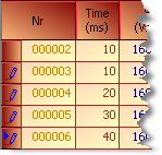
The default "Frame display time" specified in the NumericUpDown-control is used for all images imported as new frames (see "Image-Editing").
The default "Frame display time" specified in the NumericUpDown-control is applied to all frames selected in the "Frames-grid" by clicking on the Apply-button.
The second row (Magenta) encloses three buttons, which provide access to distinct dialogs or controls which offer different approaches to manipulate the timing-patterns of either selected sequences (scenes) or the whole animation. This approaches are discussed in the following sections.
Linear
The Linear-button gives access to controls, which provide the means to increment or decrement the display-time (the time, a frame remains visible in the rendered movie) of selected frames relative to their actual value in a range of +/- 2000 ms.
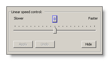
This "Linear speed control" is implemented as a TrackBar-control. The nominal range of this TrackBar is from +2000 ms to -2000 ms, or -in other words - the display-time of a given frame can be prolonged or shortened up to 2 seconds. While it is possible to always prolong a given display-time by any desired amount, this is not possible if the display-time is going to be reduced. Negative display-times (or 0) are not possible, therefore a given display-time can only be reduced to the shortest (fastest) possible display-time, which is 10 ms.
If the slider is dragged to the right, the animation gets faster, because the display-time of the affected frames is reduced. Dragging the slider to the left increments the display-time of the selected frames, slowing down the animation. The effect of this manipulations is shown in the examples below:
| Change | Result |
 |
|
 |
|
 |
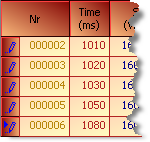
The display-time of the selected frames has been incremented by 1000 ms. |
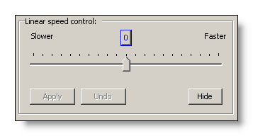
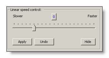
As can be seen in the examples above, as soon as the slider is moved, the previously disabled buttons (Apply and Undo) get enabled.
The Apply-button commits the new values and resets the slider to the zero-position in the center of the TrackBar, because the new values are now the base values from which to increment or decrement the display-time. Also the Apply- and Undo-buttons will be disabled again.
The Undo-button (and also the 0-button at the center of the TrackBar) will reset the display-times back to the values they had before the slider was moved.
The Hide-button finally hides the "Linear speed control"-panel.
Relative
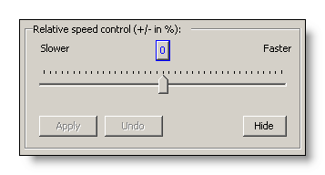
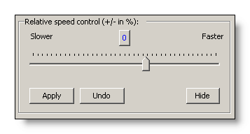
The Relative-button gives access to controls, which provide the means to increment or decrement the display-time (the time, a frame remains visible in the rendered movie) of selected frames relative to their actual value in a range of +/- 200%.
This "Relative speed control" is also implemented as a TrackBar-control. The nominal range of this TrackBar is from +200% to -200%, or -in other words - the display-time of a given frame can be prolonged or shortened up to 200 percent of its original value. As with the "Linear speed control", it is only possible to reduce display-times to the shortest (fastest) possible value of 10 ms.
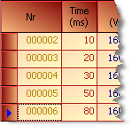
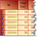
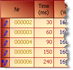
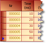
If the slider is dragged to the right, the animation gets faster, because the display-time of the affected frames is reduced. Dragging the slider to the left increments the display-time of the selected frames, slowing down the animation. The effect of this manipulations is shown in the examples below:
| Change | Result |
 |
|
 |
|
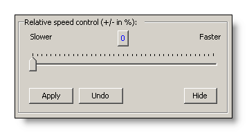 |
The display-time of individual frames has been increased by 200 percent. |
The behavior of the three buttons (Apply, Undo and Hide) is the same as described in the section on the "Linear speed control".
Accelerate
The Accelerate-button opens a more complex dialog to manipulate the display-time of the selected frames. If no frames are selected in the "Frames-grid", the changes made in this dialog will affect the whole Animation:
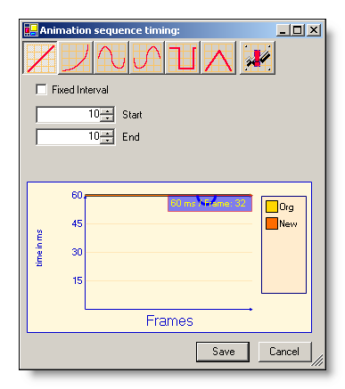
(Picture 1)
This dialog allows to apply acceleration-patterns to the display-time of the selected frames. This means, it is possible to let a whole animation - or parts of it - accelerate or slow down based on mathematical functions. To clarify the concept, we demonstrate the effects of the various acceleration-patterns applied to the same set of frames, and on the way we explain the usage of the "Animation sequence timing"-dialog.
Please note: In the rest of this section we are going to display real animated samples to illustrate the concepts discussed in the text. The animated images (the movement) are only visible in the online-help respectively the Microsoft Document-Explorer. The timing-precision and performance for animations rendered by either a Web-Browser or the Document-Explorer is not comparable to the precision achieved with the real ToolTipsFactory components. Therefore the samples may seem slower as they would be when rendered by the real components. It's also possible that the effects we want to demonstrate are not as pronounced or as smooth as they would be in the real tooltips. So, if you want to see the "real thing" you can load the sample Animation (AsysAnimationToolTipTestMovie.afx) from the "<ToolTipsFactoryHomeDir>.\Animations"-directory and repeat the experiments with the real components.
For this experiments, we'll use the Abstraction Systems logo animation, which - when animated with a static display-time of 60 ms/frame - looks as in the following movie-clip:

(Clip 1)
The chart in the lower part of the dialog (Picture 1) shows a graphical representation of the animation sequence timing (the display-time of the selected frames), where the X-axis represents the Frame-Numbers and the Y-axis the time in milliseconds between one frame and the next. This graphical representation makes it easy to see at a glance, which parts of an animation are faster and which are slower. But It is also possible to move the mouse-pointer along the drawn curve to get the exact display-time for each frame displayed in the tooltip (see Picture 1).
The timing-pattern for the sample animation (Clip 1) we are going to work on, is represented as a straight horizontal line in the chart, because all frames have the same display-time of 60 ms. This gives the animation a smooth constant movement - the logo flies around the globe at constant speed.
In the following we are going to apply some dramatic changes to the "orbital speed" of the logo with the help of the tools provided by the "Animation sequence timing"-dialog.
Linear acceleration
Before we continue, we should point out one thing, that possibly could cause some confusion: Frames with short display-times mean that there is only a short interval between the frames, thus the animation is rendered faster, while frames with higher display-times lead to a slower animation-speed.
For the first experiment, we select the Linear-button (that's the default anyway) and enter the following values as parameters for the curve:
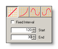 |
By selecting the
"Linear" acceleration mode, we express that we want a
constant increase or reduction in speed across the selected frames.
This constant acceleration can only be calculated if the desired DisplayTime
for the first and the last frame of the sequence are known. This
values are specified in the Start- and End-fields of the
dialog.
In order to get a constant decrease of speed (deceleration) the Start-value should be smaller then the End-value. A constant increase of speed (acceleration) is achieved with Start > End, as in our experiment, where we are going to constantly increase the speed from one frame to the next (thus reducing the display-time of the affected frames). |
As soon as the parameters are entered, the defined acceleration- or deceleration-curve can be applied to the selected frames. This is done through the Preview-button:
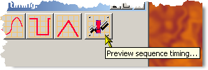 |
Clicking on this button will equally distribute the total increase of speed over the selected frames and assign the corresponding display-times to the frames. |
The new display-times are also plotted in the chart. This makes it possible to compare the old (orange) and the new (dark orange) acceleration-patterns:
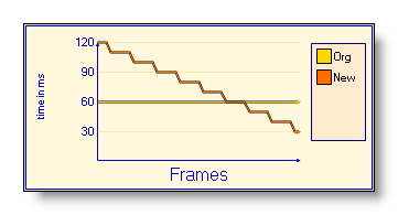 |
As becomes obvious from the graphics, the new acceleration-pattern is not what one would call "linear". But there is a simple explanation for the new curve looking like a stair: Because a fix increase of speed (90) had to be distributed over a limited number of frames (45) and the (known) resolution of the timer used to render the clips is 10 ms, the display-times where rounded to the next 10 ms-step. This rounding has the side-effect of several frames having the same display-time. This looks awkward as a plotted curve, but when the animation is finally rendered, the impression of the acceleration is quite smooth, as can be seen in Clip 2: |
If the new timing-pattern has the desired form, it can be committed by clicking on the Save-button. This will definitely apply the new values to the selected frames and the dialog will be closed. The new display-times will also be reflected in the Frames-grid. Clicking on the Cancel-button will close the dialog but leave all display-times in their original state.
As long as the dialog is open, new curves can be generated at will and compared to the original timing-pattern.
For our experiment we save the generated timing-pattern and test it in an AnimationToolTip (after saving the Animation of course). The result should look (or better: rotate!) as shown below:

(Clip 2)
Exponential acceleration
The general handling of the "Animation sequence-timing"-editor is the same as described in the section above ("Linear acceleration"), therefore it is omitted in the following and we'll concentrate on the next experiment.
This time we select the Exponential-button and enter the following values as parameters for the curve:
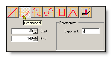 |
By selecting the
"Exponential" acceleration mode, we express that we want an
exponential increase or reduction in speed across the selected frames.
An exponential acceleration can only be calculated if the DisplayTime
of the Start- and the End-frame of the sequence, and the
desired Exponent as well, are known. This values are specified
in the according fields of the dialog.
Again: In order to get a decrease of speed (deceleration) the Start-value should be smaller then the End-value, as in our experiment, where we are going to exponentially slow down the speed from one frame to the next (thus increasing the DisplayTime of the affected frames). An increase of speed (acceleration) is achieved with Start > End. |
As soon as the parameters are entered, we can get the new acceleration-pattern by clicking the Preview-button:
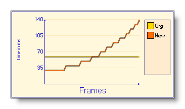 |
Again, the
resulting shape looks more as a stair, because of the limited
resolution of the animation-timer, which makes it necessary to round
the display-times to the next 10 ms boundary.
But despite of this stair-effect, the exponential character of the curve becomes obvious - the deceleration is small at the beginning and starts only to increase substantially in the second half of the Animation. |
If this curve is applied to the Animation, a noticeable slow-down should be noted in the "orbiting" logo (Clip 3). And, because the clip is played endlessly, a sudden acceleration should be noted as well, as soon as the animation starts over. (This is the case because at the beginning the Animation is quite fast and at the end massively slowed down, which leads to a sudden change in speed, when the animation starts over.)

(Clip 3)
Sine and Cosine acceleration-pattern
The Sine and Cosine acceleration patterns are basically identical to use. Therefore we'll discuss only one of them in this chapter.
For this experiment we select the Sine-button and enter the following values as parameters for the curve:
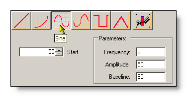 |
By selecting the
"Sine" or the "Cosine" acceleration mode, we
express that we want an oscillating increase and reduction in
speed across the selected frames. A sinusoidal or cosinusoidal
acceleration can only be calculated if at least an Amplitude
(the amount of oscillation to both sides of the Baseline) and a
Baseline (the center of the oscillation) are given. Another
important parameter that should be provided is the Frequency,
which defines how many complete oscillations have to be
calculated.
The Start-parameter allows to define a display-time from which the curve should start. This means, the sine-wave is shifted to the left until the point on the curve with this value (display-time) crosses the first frame. This implicates that the defined Start-value must adhere to the following rule: (Baseline-Amplitude) < Start < (Baseline+Amplitude) |
As soon as the parameters are entered, we can get the new acceleration-pattern by clicking the Preview-button:
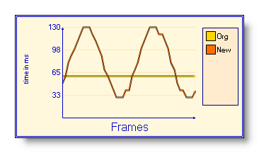 |
This time we get a nicely shaped sinusoidal curve, which oscillates twice in the specified range. The errors (or deformations) due to the needed rounding are minimal this time. |
If this curve is applied to the Animation, the periodical deceleration/acceleration-cycles should be clearly visible in the "orbiting" logo (Clip 4). And, because the curve ends with the same display-time as it started, there should be no abrupt velocity-changes when the clip starts over if played endlessly.

(Clip 4)
Rectangular acceleration-pattern
The rectangular acceleration-pattern is similar to the Sine and Cosine acceleration patterns. It is selected through the Rectangular-button:
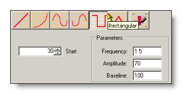 |
By selecting the
"Rectangular" acceleration mode, we express that we want an
alternating speed across the selected frames. Such a rectangular
acceleration-curve can only be calculated if at least an Amplitude and
a Baseline (the center of the oscillation) are given. And - as
for the sine and cosine curves - the Frequency is also an
important parameter that should be provided. It defines how many times
the display-time should alternate between the low (Baseline-Amplitude)
and the high value (Baseline+Amplitude).
The Start-parameter allows to define a display-time from which the curve should start. This means, the rectangular wave e is shifted to the left until the point on the curve with this value (display-time) crosses the first frame. This implicates that the defined Start-value must adhere to the following rule: (Baseline-Amplitude) < Start < (Baseline+Amplitude) In practice, with the Start-value it is possible to define, whether the curve starts with the high display-time (slower animation) or the low one (faster). |
As soon as the parameters are entered, we can get the new acceleration-pattern by clicking the Preview-button:
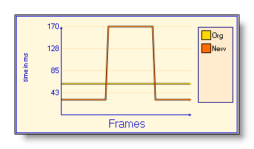 |
This time we get a nicely shaped rectangular curve, which oscillates exactly 1.5 times between the low and the high display-time. |
If this curve is applied to the Animation, the fast and the slow -cycles should be clearly distinguishable in the "orbiting" logo (Clip 5). And, because the curve again ends with the same display-time as it started, there should be no abrupt velocity-changes when the clip starts over if played endlessly.

(Clip 5)
Triangular acceleration-pattern
|
The triangular acceleration-pattern is similar to the Sine, Cosine and Rectangular acceleration patterns. It is selected through the Triangular-button. The usage is identical to the Sine, Cosine and Rectangular patterns. |